Paper Explanation: Faster R-CNN Towards Real-Time Object Detection with Region Proposal Networks

What Led to Faster R-CNN?

Even though networks like Fast R-CNN achieve a really high accuracy, they are very slow to be of practical use in real time. The reason for such slow speeds is the region proposal step in the architecture! Algorithms, like Selective Search (used in Fast R-CNN) take around 2 seconds per image to generate region proposals. This is far from practical. As a result, region proposals become the test-time computational bottleneck in state-of-the-art detection systems!

Solution

Let’s just use CNNs for computing region proposals as well! Not only this, but the same convolutional layers can be used to generate region proposals as well as for detection. By sharing convolutions at test-time, the marginal cost for computing proposals is small (around 10ms per image!).

To calculate region proposals using CNN Region Proposal Network (RPN) were introduced.

The Architecture of Faster R-CNN

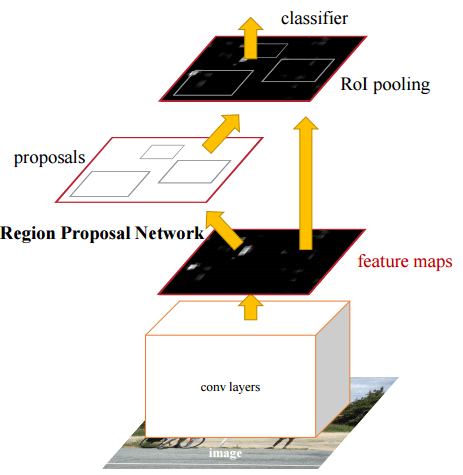
Faster R-CNN is composed of two modules:

1. The first is a deep fully convolutional network that proposes regions.
2. The second is just Fast R-CNN which uses the region proposals given by the first part (instead of those by selective search used in the Fast R-CNN paper).

In this post I will not go over the Fast R-CNN part of the network and mainly focus on the new novel Region Proposal Networks (RPNs). To understand Fast R-CNN, please refer to this post.

The input image is re-scaled such that its shorter side is 600 pixels. The re-scaled image is then passed through a deep convolutional neural network (such as VGG16 or ZF). This gives the feature map. The region proposal network uses the feature map to generate region proposals (like the name suggests).  After this, the region proposals and the feature map is passed onto the RoI pooling layer (from here on it is the Fast R-CNN architecture). Finally, the output of the RoI pooling layer goes to a classifier and a bounding-box regressor which give us the class label and the detection window respectively.

The above was just a quick overview of the architecture. Now let’s dive deeper to understand the Region Proposal Network!

Region Proposal Networks (RPNs)

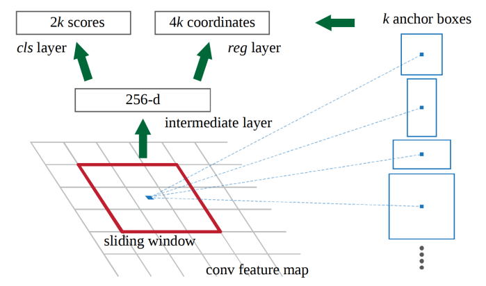
The job of this is to output a set of rectangular object proposals, each with an “objectness” score.

The RPN, acts on the feature map generated by the deep CNN and takes as input an n × n (In the paper n = 3 is used) spatial window of the feature map. The RPN network is slid over the whole feature map. At each sliding-window location, multiple region proposals are simultaneously predicted. The maximum number of possible proposals for each location is k.

The RPN can be thought of as a 3 × 3 dimensional “block” that slides over the whole feature map using stride = 1. Also, the feature map is zero padded with padding = 1. This allows each pixel in the original feature map (without padding) to be the center of the 3 × 3 region.

What are Anchors?

The k proposals are parameterized relative to k reference boxes, called anchors. An anchor is centered at the sliding window and is associated with a scale and aspect ratio. Generally, 3 scales and 3 aspect ratios are used, giving k = 3 * 3 = 9 anchors at each sliding position (and hence  9 region proposals). The scales with box areas of 128², 256² and 512² are used and the aspect ratios of 1:1, 1:2 and 2:1 are used.

Now hang on a minute! You might be wondering, aren’t the anchor boxes too big? For a typical 1000 × 600 image, the size of the feature map will be around 60 × 40. There is no way those anchor boxes are fitting!

WRONG!

This is because the anchor boxes are applied on the original input image and not on the feature map!

Now let’s get back to the RPN. (In the coming section, I have taken ZF to be the deep CNN used. If VGG16 is taken instead, instead of 256, it becomes 512 in the following discussion).

The RPN can be taken to be composed of the following sub-parts:

1. A convolutional layer using  n × n size filters. The number of such filter used in the layer is 256. An important point to take note is that, this convolution is being done on the n × n input to the RPN. Hence the output of the above convolution is a 1 × 1 × 256 feature map (can also be called a 256-d feature vector).
2. A classification layer that takes as input this feature map and outputs the probabilities of a particular proposal being an object or not. This is a class agnostic layer and thus only gives the information of the presence of an object or not. This layer will give 2k scores. 2 scores for each region proposal and there are k region proposals (for k anchors). This is implemented as 2 * k , 1 × 1 convolutions on the feature map.
3. A regression layer outputs 4 numbers for each region proposal, hence it outputs 4 * k numbers. These 4 numbers give offsets that help refine and adjust each anchor box to get final region proposals. This is implemented as 4 * k,  1 × 1 convolutions on the feature map. These output numbers are with respect to the input image!

All of the above process is just for one input of the RPN. As the RPN is slid across the whole feature map as was previously explained, the above mentioned process repeats all over again for each position.

As a result we will end up having roughly 20000 (≈ 60 x 40 x 9) anchors (and thus region proposals).

Intuition of how RPN works

What is a region proposal? It is just 4 numbers!

Let me elaborate.

Instead of thinking of a region proposal as portion of the whole image, it is better to think of them as 4 numbers (though both give the same thing): coordinates of the center and the height and width of the proposal. Hence, it is the regression layer in the RPN that actually generates the proposals. The 4k output of the regression layer should be thought of as k groups of 4, where, each group gives 1 region proposal.

The purpose of the classification layer is to help us classify each region proposal as foreground (it is an object) or background (not an object). Again, the 2k outputs should be divided into k groups of 2 where each group helps us classify one particular region proposal.

Training of Faster R-CNN

Training RPN

It can be trained end-to-end by back-propagation and stochastic gradient descent.

A binary class label (of being an object or not) is assigned to each anchor. A positive label is defined is assigned to:

1. Anchors with the highest IoU overlap with a ground-truth box
2. Anchors that have an IoU overlap higher than 0.7 with any ground-truth box.

Usually the second condition is sufficient to determine the positive samples but the first condition is still used in case some rare case occurs where no positive proposals are found by the second condition.

A negative label (background) is assigned to a non-positive anchor is its IoU ratio is lower than 0.3 for all ground-truth boxes.

Anchors that are neither positive nor negative do not contribute to the training!

The loss function is defined as:

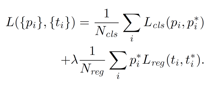
i  =  index of an anchor in a mini-batch

pi  =  predicted probability of anchor i being an object.

pi*  =  ground-truth label; 1 if anchor is positive and 0 if negative

ti  =  vector representing the 4 parameterized coordinates of the predicted bounding box associated with a positive anchor

ti*  =  vector representing the 4 parameterized coordinates of the ground-truth box associated with a positive anchor

The classification loss (first term) is log loss over two classes. For the regression loss (second term), smooth L1 loss is used.

For bounding box regression, the following paramaterization of the 4 coordinates is adopted:

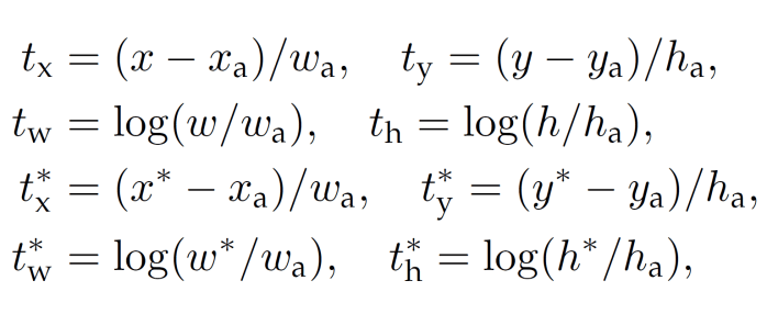
Variables x, xa, and x* are for the predicted box, anchor box and ground-truth box respectively (similarly for y, w, h).

Mini-Batch Used

Each mini-batch arises from a single image that contains many positive and negative example anchors.

256 anchors are randomly sampled from an image, where the sampled positive and negative anchors have a ratio of up to 1:1. If there are fewer than 128 positive samples, negative samples are added to make the mini-batch size 256.

Anchor boxes that cross image boundaries are ignored.

4-step Alternating Training

As is obvious from the name, the process consists of 4 steps:

1. Train the RPN as described above. The network is initialized with an ImageNet-pre-trained model and fine-tuned end-to-end for the region proposal task.
2. Train a separate detection network by Fast R-CNN using the proposals generated by the RPN trained in step-1. This detection network is also initialized with an ImageNet-pre-trained model.
3. Use the detector network trained in step-2 to initialize RPN training but fix the shared convolutional layers (do not train) and only fine-tune the layers unique to RPN. (Now the RPN and detector share convolutional layers)
4. Keeping the shared convolutional layers fixed, fine-tune the unique layers of Fast R-CNN (the detector).

The above training process is very messy! There are methods for jointly training everything together (RPN + Fast R-CNN) described in the paper. I will not go into them in this post. You can read about them in the original paper.

Test Time

The fully convolutional RPN is applied to the entire image. Any cross-boundary proposal boxes are clipped to the image boundary (not ignored as was done during training). Non-Maximum Suppression (NMS) is applied on the proposals based on their class scores. The NMS threshold is set at 0.7. This leaves us about 2000 proposals per image. After NMS, only the top-N (N can be as low as 300 without affecting performance) ranked proposals are used for detection.

Conclusion

Faster R-CNN is basically a Fast R-CNN which uses RPN instead of selective sea rch for region proposals. By sharing convolutional features the region proposal step becomes nearly cost free. Also, as the learned RPN improves region proposal quality and this helps boost up the overall object detection accuracy.

Link to the paper: https://arxiv.org/abs/1506.01497

 

Mohit Jain