Called Fast R-CNN because it’s comparatively fast to train and test.
Why Fast R-CNN?
Even though R-CNN had achieved state of the art performance on object detection it had many problems:
- Slow at test-time due to independent forward passes of the CNN for each region proposal.
- The CNN doesn’t get trained during the training of the SVM classifiers and bounding box regressors.
- Complex multi-stage training pipeline.
To solve the above problems, Fast R-CNN comes in. It not only gave the state of the art performance on detection but also made everything else better:
- Training is single-stage, using multi-task loss.
- Training can update all the network layers.
- Fast at test time (hence, the name!)
Now let’s look at the network architecture.
Fast R-CNN Architecture

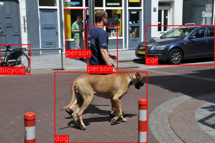
The Fast R-CNN network takes as input an entire image (original high resolution image without and downscaling) and a set of object proposals. The object proposals can be calculated using methods like selective search.
The image is forward propagated through a convolutional neural network such as VGG16. This produces a feature map.
After this, for each object proposal, a region of interest (RoI) pooling layer extracts a fixed-length feature vector from the feature map.
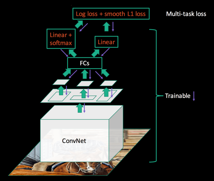
Each feature vector is now fed into a sequence of fully connected (fc) layers that finally branch off into two sibling output layers:
- One the produces softmax probability and estimates over K object classes plus an additional “background” class.
- A second layer that outputs four real-valued numbers for each of the K object classes. These 4 values give the refined bounding-box position.
What is the RoI pooling layer?
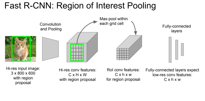
This is basically a max pooling layer that, contrary to a normal max pooling layer, works on different dimensions of inputs. In other words, you can say it has “adaptable” filter dimensions. The job of this layer is to convert the features inside any valid region of interest into a small feature map with a fixed spatial extent of H × W (H = W = 7 for VGG16). Here, H and W are hyper-parameters that are independent of any particular RoI.
The reason to confine the output to a fixed spatial dimension of H × W is that the fully connected (fc) layers cannot work on different dimensional inputs (like a convolutional layer can). Thus, on flattening the C × H × W (C is the number of channels) feature map should give the expected input dimensions of the fc layer.
What is a Region of Interest (RoI)?
RoI is a rectangular window into a conv feature map.
When an image is forward propagated through a CNN, it’s dimensions get reduced, i.e: the image gets “scaled down”. A 128 × 128 input image may give a 7 × 7 final conv feature map (output dimensions depend on the network used). For object detection in Fast R-CNN the same method employed by R-CNN is used, i.e: finding the feature map for each object proposal, but doing it by sharing computation! To do this, the object proposal gets scaled down by the same factor as the overall image to give the region of interest (RoI). In other words, the projection of the object proposal onto the conv feature map gives the region of interest (RoI).
Each RoI is defined by a four-tuple (r, c, h, w) that specifies its top-left corner (r, c) and its height and width (h, w).
How does RoI pooling work?
RoI max pooling works by dividing the h × w RoI window into an H × W grid of sub-windows of approximate size h/H × w/W and then max-pooling the values in each sub-window into the corresponding output grid cell, i.e. the “max-pooling” filter size becomes h/H × w/W. Pooling is applied how it is normally applied, independently to each feature map channel.
Training of Fast R-CNN
A pre-trained ImageNet network is used to initialise the Fast R-CNN. Three transformation are done thereafter:
- The last max pooling layer is replaced by a RoI pooling layer that is configured by setting H and W to be compatible with the net’s first fully connected layer.
- The network’s last fully connected layer and softmax are replaced with two sibling layers: a fully connected layer and softmax over K + 1 categories and category-specific bounding-box regressors.
- The network is modified to take two data inputs: a list of images and a list of RoIs in those images.
Fine-Tuning for Detection
All the network weights are trained with back-propagation.
Stochastic gradient descent (SGD) mini-batches are sampled hierarchically, first by sampling N images and then by sampling R ⁄ N RoIs from each image. One thing to note is that, RoIs from the same image share computation and memory. This is because RoIs for a particular image will all come from the same conv feature map.
Fast R-CNN has only one fine-tuning stage (R-CNN has three) that jointly optimizes a softmax classifier and bounding-box regressors. It is able to do this by using a multi-task loss.
Multi-Task Loss
The first layer outputs a discrete probability distribution (per RoI), p, over K+1 classes. The second layer outputs bounding-box regression offsets, tk, for each of the K objects classes. tk specifies a scale-invariant translation and log-space height/width shift relative to an object proposal.
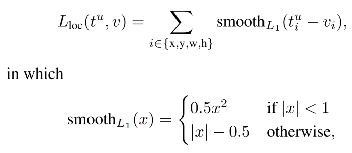
The multi-task loss is defined as:

The first term is the log loss for true class u.
The second term is the loss for the bounding-box regressor. It is basically a smooth L1 Loss. [u ≥ 1] is called the Iversion bracket indicator function which evaluates to 1 when u ≥ 1 and 0 otherwise. By convention, the background class is labelled as u = 0. This is done because, there is no meaning in having a bounding box for a background RoI.
λ is a hyperparameter that controls the balance between the two task losses.
Mini-Batch Sampling
Each SGD mini-batch is constructed from N = 2 images, chosen uniformly at random. The mini-batch size is R = 128. 64 RoIs are sampled from each of the two images. 25% of the RoIs with IoU intersection over union (IoU) overlap with ground-truth box ≥ 0.5 constitute the positive class i.e: u ≥ 1. The remaining RoIs are sampled from object proposals that have maximum IoU with the ground truth in the interval [0.1, 0.5).
Other than horizontally flipping the images with a probability of 0.5, no other data augmentation is used during training.
Detection using Fast R-CNN
The image along with R object proposals are given as input. During testing, R is typically around 2000 (during training it was 128!). For each test RoI r (∈ R), the forward pass outputs a class posterior probability, P(class | r), distribution p, and a set of bounding-box offsets relative to r. A detection confidence is assigned to r for each class. Finally, non-maximum suppression is performed independently for each class.
Some more contributions of the paper:
- Softmax perform better than SVMs
- Multi-task training helps improve even just pure classification accuracy relative to training for classification alone.
Link to the paper: https://arxiv.org/pdf/1504.08083.pdf
