A Look at Image Segmentation using CNNs

Image segmentation is the task in which we assign a label to pixels (all or some in the image) instead of just one label for the whole image. As a result, image segmentation is also categorized as a dense prediction task. Unlike detection using rectangular bounding boxes, segmentation provides pixel accurate locations of objects in an image. Therefore, image segmentation plays a very important role in medical analysis, object detection in satellite images, iris recognition, autonomous vehicles, and many more tasks.

With the advancements in deep learning methods, image segmentation has greatly improved in the last few years; in terms of both accuracy and speed. We can now generate segmentations of an image within a fraction of a second and still be very accurate and precise.

The Goal of this Post

Through this post, we’ll cover the intuition behind some of the main techniques and architectures used in image segmentation. We’ll start with semantic segmentation and later move on to instance segmentation. More weight will be on the instance segmentation techniques as these are a more advanced version of the segmentation task (combining detection with segmentation).

Let’s start!

Semantic Segmentation

Semantic image segmentation is the task that assigns every pixel in the image a semantic category label. It does not distinguish between object instances. Tackling this task has been handled majorly by the family of approaches based on FCNs. Now let’s look at some of the methods used.

Fully Convolutional Networks (FCNs) [1]

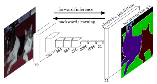
To create an FCN, just replace all the fully-connected layers of a CNN (such as VGG, etc.) to 1×1 convolutions. The number of filters of this convolutional layer will be equal to the number of neurons (outputs) of the fully-connected layer. This is done because, for segmentation, the spatial location of each pixel is important and conv. layers are naturally able to handle this whereas fully-connected layers fail. As a result, locations in higher layers correspond to the locations in the image they are path-connected to, i.e. their receptive fields.

The FCN architecture is very simple and consists of an encoder CNN (VGG is used in the paper) with all fully-connected layers appropriately transformed as described earlier. To this, an additional convolutional layer is appended consisting of N+1, 1×1 filters, where N is the number of classes and the extra one is for the background. This completes the encoder network of FCN. As can be seen, the number of channels in the output feature map of the encoder is N+1.
The encoder is followed by the decoder network. This consists of only a single backward convolutional layer (sometimes also called transposed convolution or deconvolution). The output is of the same spatial dimensions as the input image and has N+1 channels. Each channel predicts the segmentation mask for one class only. Backward convolution is convolution with fractional input stride of  1 ⁄ f, where f is the upsampling factor. Implementing it is simply reversing the forward and backward passes of a normal convolution.

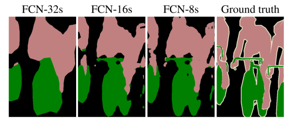
Taking VGG as the main convolutional network: as features of the last pool-5 layer are coarse, features of pool-4 and pool-3 are also used. This helps to generate better segmentations by better delineating the boundaries. All of these features are combined as shown in the following figure:

One thing to note is that all the pooling features used are first passed through a conv. layer with N+1, 1×1 filters before getting upsampled.

U-Net [2]

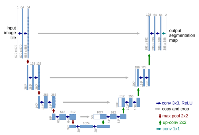
This model is mainly used for medical image data. It also follows the encoder-decoder structure of FCNs. It also doesn’t use any fully-connected layers. The encoder is just normal a convolution network consisting of 10 conv. layers with max-pooling layers in between.
The decoder consists of upsampling the feature map and performing normal convolutions on it multiple times. The upsampling is performed using backward convolutions consisting of 2×2 filters and the output has half the number of channels as the input. The final conv. layer of the decoder is a 1×1 conv. layer that gives an output with channels equal to the number of classes plus background. In total there are 13 conv. layers (including backward conv. layers) in the decoder network. Hence, the whole architecture consists of 23 learnable conv. layers.

An additional step in the decoder is the concatenation of the corresponding encoder feature map (before max-pooling) with the upsampled output in the decoder. This is done to account for the background information that gets lost during the pooling operation.

SegNet [3]

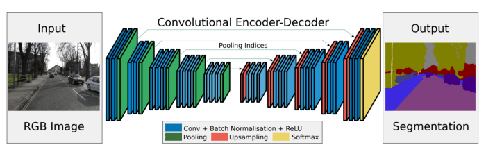
The SegNet architecture also follows the encoder-decoder pattern. In fact, most semantic segmentation architectures have the same basic pattern! The encoder of the network is a fully convolutional VGG16. The decoder is very similar to that of U-Net: there is repeated upsampling followed by convolutions. However, there are some important key differences:

• The upsampling is not learnable.
• The decoder network has the same type of convolutions as the encoder (filter sizes and channels of corresponding layers are same).

The upsampling step in SegNet is a sort of backward max-pooling operation. During the forward pass in the encoder, the max-pooling indices are stored, i.e. the location of the highest value pixel in the 2×2 max-pooling window at each sliding position of the layer. These are then used for upsampling in the decoder (the corresponding upsampling step to the max-pool in the encoder). The remaining pixels in the upsampled output are set to zero.

Normal convolutions are performed on this sparse feature map to produce a dense feature map. This is in contrast to what is done in U-Net, where the whole encoder feature map is stored which requires larger memory for storing the floating point values of the feature map. On the other hand, the max-pooling indices used in SegNet can be very efficiently stored using just two bits!
Hence, the decoder network of SegNet consists of a hierarchy of decoders, one corresponding to each encoder and the appropriate decoder uses the max-pooling indices from the corresponding encoder to perform non-linear upsampling of their input feature maps.

One thing to note is that the decoder corresponding to the first encoder (closest to the input image) produces a multi-channel feature map, although its encoder input has 3 channels (RGB). This is unlike the other decoders in the network which produce feature maps with the same number channels and size as their encoder inputs. This is done for generating the segmentation masks for each class plus background.

Now let’s move onto instance segmentation.

Instance-Aware Semantic Segmentation

This task requires both classification and segmentation of object instances. This is different, and essentially more complex, compared to the previous task which doesn’t distinguish between the different instances of the same class. Methods used to tackle this problem generally create individual diminished masks for each object which are then resized to the size of the object in the input image. This is also in contrast to the methods used to handle the previously discussed which output a segmentation of the whole image with the same size.
Now let’s look at some of the techniques used for Instance-Aware Semantic Segmentation.

DeepMask [4]

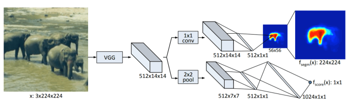
This method creates a segmentation mask of dimensions 56×56 of the object centered at the image patch given as input and also classifying it. For the input patch to give a segmentation, it should satisfy the following constraints:

1. the patch contains an object roughly centered in it
2. the object is fully contained in the patch and in a given scale range

As the DeepMask method only segments one object per patch, it is applied densely at multiple locations and scales of the whole image. This is necessary so that for each object in the image, at least one patch is tested that satisfies the above two constraints.

The architecture consists of the VGG-A network with all the fully-connected layers and the last max-pooling layer removed. The output of this has a downsampling factor of 16. This is then fed into two parallel branches: one for predicting the class (score) and the other for generating the masks.

The score branch consists of a 2×2 max-pooling layer followed by two fully-connected layers with 512 and 1024 hidden units respectively. Both of these layers use a ReLU non-linearity and dropout with a probability of 0.5. A final linear layer then generates the object-score.
The segmentation branch begins with a single 1×1 conv. layer with 512 filters. The output feature map is fully connected to a low dimensional output of size 512, which is further fully connected to each pixel classifier to generate an output of dimensions 56×56. A bilinear upsampling layer is used to transform this output to the resolution of the input image patch.

DeepMask, while being a decent segmentation method, can also be used to generate object proposals to replace methods like Selective Search which is not trainable and hence has limited performance.

Multi-task Network Cascades (MNC) [5]

Instead of tackling the instance-aware semantic segmentation task straight on as a whole, this method breaks it down into three smaller and simpler sequential sub-tasks:

1. Differentiating instances. This sub-task essentially predicts bounding-boxes and objectness probability for each instance.
2. Estimating masks. A pixel-level mask is predicted in this sub-task.
3. Categorizing objects. In this sub-task, the category-wise label is predicted for each mask-level instance.

Instead of performing these sub-tasks in parallel, they are cascaded one after the other, hence, the name.

VGG-16 with all fully connected layers removed is used to create a feature map of the input image which is then shared with all the three sub-tasks.

Sub-Task 1: Regressing Box-Level Instances
The network proposes object instances in the form of bounding boxes. These bounding boxes are class-agnostic and are predicted with an objectness score (probability of containing an object or not). The network structure is similar to the Region Proposal Networks (RPNs). To read about them check out my post on Faster R-CNN.

Sub-Task 2: Regressing Mask-level Instances
Using a box prediction given by stage-1, a feature of this box is extracted from the shared convolutional features using Region-of-Interest (RoI) pooling. This is then passed through two fully-connected layers. The first fc layer reduces the dimensions to 256, followed by the second fc layer that regresses a pixel-wise mask. The mask is of a predefined spatial resolution of m×m (= 28), which is parametrized by an m²-dimensional vector. This is similar to the mask prediction method used in DeepMask. DeepMask applies the regression layers to dense sliding windows (fully-convolutionally), but MNC regresses masks only from a few proposed boxes and so computational cost is greatly reduced.

Sub-Task 3: Categorizing Instances
Just like stage-2, using the box predictions given by stage-1, a feature map is extracted using RoI pooling. This is followed by two parallel pathways: mask-based and box-based.
In the mask-based pathway, the RoI extracted feature map is “masked” by the stage-2 mask predictions. This leads to a feature focused on the foreground of the prediction mask. Two 4096-d fc layers are applied to the masked feature. The box-based pathway simply consists of the feature extracted using RoI pooling being passed through to 4096-d fc layers.  The box-level pathway is for addressing the cases when the feature is mostly masked out by the mask-level pathway (eg., on background or very big objects). The mask-based and box-based pathways are concatenated followed by a softmax classifier for predicting N+1 classes: N categories plus one background category.

Even after using such a complex architecture, the whole network is end-to-end trainable!

InstanceFCN [6]

This method adapts FCNs, which perform really well for semantic segmentation, for instance-aware semantic segmentation. In contrast to the original FCN where each output pixel is a classifier of an object category, in InstanceFCN each output pixel is a classifier of relative positions of instances. For example, for the #6 score map in the figure below, each pixel is a classifier of being or not being “right side” of an instance.

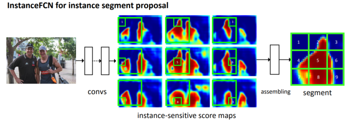
An FCN is applied on the input image to generate k² score maps, each corresponding to a particular relative position. These are called instance-sensitive score maps. To produce object instances from these score maps, a sliding window of size m×m is used. The m×m window is divided into k², m ⁄ k × m ⁄ k dimensional windows corresponding to each of the k² relative positions. Each m ⁄ k × m ⁄ k sub-window of the output directly copies values from the same sub-window in the corresponding score map. The k² sub-windows are put together according to their relative positions to assemble an m×m segmentation output. For example, the #1 sub-window of the output in the figure above is taken directly from the top-left m ⁄ k × m ⁄ k sub-window of the m×m window in the #1 instance-sensitive score map. This is called the instance assembling module.

The architecture consists of applying VGG-16 fully convolutionally on the input image. On the output feature map, there are two fully convolutional branches; one for estimating segment instances (as described above) and the other for scoring the instances.

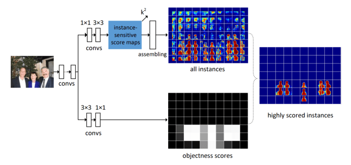
For the first branch, 1×1 512-d conv. layer followed by a 3×3 conv. layer is used to generate the set of k² instance-sensitive score maps. The assembling module (as described earlier) is used to predict the m×m (= 21) segmentation mask.
The second branch consists of a 3×3 512-d conv. layer followed by a 1×1 conv. layer. This 1×1 conv. layer is a per-pixel logistic regression for classifying instance/not instance of the m×m sliding window centered at this pixel. Hence, the output of the branch is an objectness score map in which one score corresponds to one sliding window that generates one instance. Hence, this method is blind to the different object categories.

FCIS [7]

Fully Convolutional Instance-aware Semantic Segmentation (FCIS) is build up of the IntanceFCN method. InstanceFCN is only able to predict a fixed m×m dimensional mask and could not classify the object into different categories. FCIS fixes all of that by predicting different dimensional masks while also predicting the different object categories.

Joint Mask Prediction and Classification

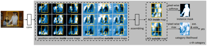
Given a RoI, the pixel-wise score maps are produced by the assembling operation as described above under InstanceFCN. For each pixel in ROI, there are two tasks (hence, two score maps are produced):

1. Detection: whether it belongs to an object bounding box at a relative position (detection+) or not (detection-).
2. Segmentation: whether it is inside an object instance’s boundary (segmentation+) or not (segmentation-).

Based on these, three cases arise:

1. high inside score and low outside score: detection+, segmentation+
2. low inside score and high outside score: detection+, segmentation-
3. both scores are low: detection-, segmentation-

For detection, max operation is used to differentiate the cases 1 and 2 (detection+) from case 3 (detection-). The detection score of the whole ROI is obtained via average pooling over all pixels’ likelihoods followed by softmax operator across all the categories.
For segmentation, softmax is used to differentiate case 1 (segmentation+) from the rest (segmentation-). The foreground mask of the ROI is the union of the per-pixel segmentation scores for each category.

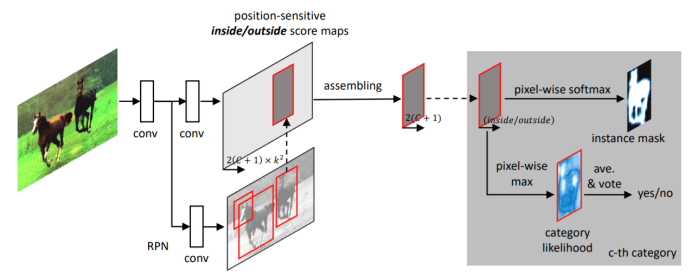
ResNet is used to extract the features from the input image fully-convolutionally. An RPN is added on top of the conv4 layer to generate the ROIs. From the conv5 feature map, 2k² × C+1 score maps are produced (C object categories, one background category, two sets of k² score maps per category) using a 1×1 conv. layer. The RoIs (after non-maximum suppression) are classified as the categories with the highest classification scores. To obtain the foreground mask, all RoIs with intersection-over-union scores higher than 0.5 with the RoI under consideration are taken. The mask of the category is averaged on a per-pixel basis, weighted by their classification scores. The averaged mask is then binarized.

Mask R-CNN [8]

Mask R-CNN is an upgrade from the Faster R-CNN model in which another branch is added in parallel with the category classifier and bounding box regressor branches to predict the segmentation masks. The mask branch consists of an FCN on top of the shared feature map that gives a Km²-dimensional output for each RoI, encoding K binary masks of resolution m×m, one for each of the K classes. This allows the network to generate masks for every class without competition among the classes. The class predicted by the classification branch is used to select the appropriate mask. This decouples the mask and class predictions.

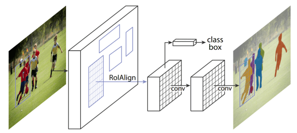
To predict accurate masks requires the spatial structure of the input image to be followed closely which convolutions are good at. However, this pixel-to-pixel behavior also requires the RoI features (which themselves are small feature maps) to be well aligned. RoIPool used to extract these features, however, isn’t always faithful to the alignments. The reason being that the dimensions of the RoI doesn’t have to be integrals but can also take on floating number numbers. RoIPool quantizes these dimensions by rounding them to the nearest integer. Not only this but the quantized RoI is further subdivided into quantized spatial bins over which pooling is performed. These quantizations affect the pixel-to-pixel alignment with the RoI and the extracted RoI features causing errors in predicting the segmentation masks.

RoIAlign

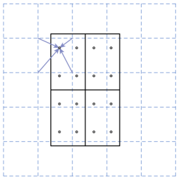
To solve this problem, a new way to extract the features, called RoIAlign, is introduced. The idea behind it is that as quantizations are causing misalignments, avoid all quantizations! For example, say the projection of the RoI on the extracted feature map is of dimensions 2.86 × 5.12. RoIPool would quantize this to 3 × 5, causing misalignments. On the other hand, RoIAlign will not do anything and use the dimensions 2.86 × 5.12 as it is. The RoI is further subdivided into smaller spatial bins (just like RoIPool) without any quantizations. Now each smaller bin may contain fractions of pixels and thus performing pooling operations will be absurd. Instead, binary interpolation is used to compute the values of the input feature at four fixed locations in each smaller bin and aggregated using max or average. One thing to note is that the RoI features extracted using RoIAlign are of fixed spatial dimensions just like that of RoIPool.

The masks predicted are always of fixed dimensions, m×m, but are resized to the RoI size and binarized.

Conclusion

For semantic segmentation, generally, variations of FCNs are used. Even in these, more focus is put on the decoder part of the network, the encoder being just a simple feature extractor.

However, many different methods have been tried to address the instance-aware semantic segmentation task. Of course, FCNs still remain an integral part but methods based on modifying detection tasks for segmentation also give good if not better results (Mask R-CNN vs FCIS).

Mohit Jain

 

References

[1]  J. Long, E. Shelhamer, and T. Darrell. Fully convolutional networks for semantic segmentation. In CVPR, 2015. (paper)

[2]  O. Ronneberger, P. Fischer, and T. Brox, “U-net: Convolutional networks for biomedical image segmentation,” in MICCAI, pp. 234–241, Springer, 2015. (paper)

[3]  Badrinarayanan, V., Kendall, A., & Cipolla, R. (2017). SegNet: A Deep Convolutional Encoder-Decoder Architecture for Image Segmentation. IEEE Transactions on Pattern Analysis and Machine Intelligence, 39, 2481-2495. (paper)

[4]  P. O. Pinheiro, R. Collobert, and P. Dollar. Learning to segment object candidates. In NIPS, 2015. (paper)

[5]  Dai, J., He, K., Sun, J. Instance-aware semantic segmentation via multi-task network cascades. In CVPR., 2016. (paper)

[6]  J. Dai, K. He, Y. Li, S. Ren, and J. Sun. Instance-sensitive fully convolutional networks. In ECCV, 2016. (paper)

[7]  Y. Li, H. Qi, J. Dai, X. Ji, and Y. Wei. Fully convolutional instance-aware semantic segmentation. In CVPR, 2017. (paper)

[8]  K He, G Gkioxari, P Dollár, R Girshick. Mask R-CNN. In ICCV, 2017. (paper)