Variational Autoencoder Explained

Variational encoders (VAEs) are generative models, in contrast to typical standard neural networks used for regression or classification tasks. VAEs have diverse applications from generating fake human faces and handwritten digits to producing purely “artificial” music.

This post will explore what a VAE is, the intuition behind it and also the tough looking (but quite simple) mathematics that powers this beast!

But first, let’s look at simple autoencoders in brief.

A Glance at Autoencoders

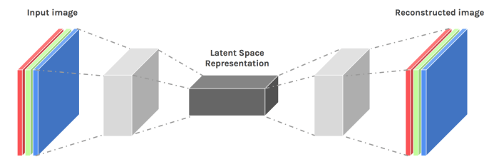
An autoencoder takes some data as input and discovers some latent state representation of the data. The encoder network takes in the input data (such as an image) and outputs a single value for each encoding dimension. The decoder takes this encoding and attempts to recreate the original input. Autoencoders find applications in tasks such as denoising and unsupervised learning but face a fundamental problem when faced with generation.

The latent space to which autoencoders encode the input to may not be continuous. Due to the discontinuity, a point sampled from there and passed to the decoder can generate unrealistic outputs. Autoencoders are only good at generating outputs of data they have already seen but face problems while trying to generate new unseen data.

Variational Autoencoders to the Rescue

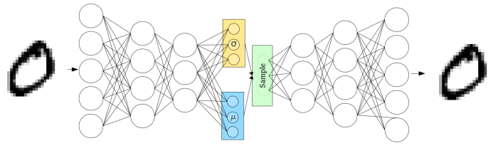
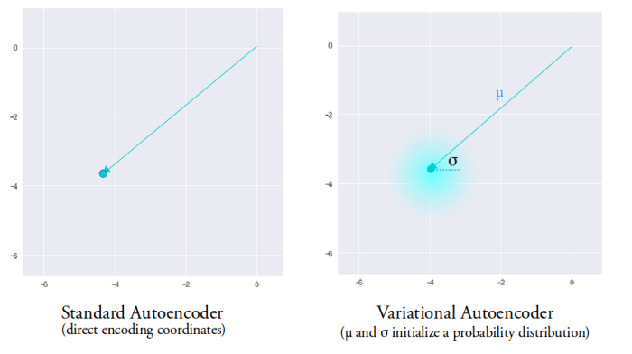
Unlike the normal autoencoders, the encoder of the VAE (called the recognition model) outputs a probability distribution for each latent attribute. For example, assume the distribution is a normal distribution. The output of the recognition model will be two vector: one for the mean and the other for the standard deviation. The mean will control where the encoding of the input should be centered around while the standard deviation will control how much can the encoding vary from the mean. To decode, the values of each latent state is randomly sampled from the corresponding distribution and given as input to the decoder (called the generation model). The decoder then attempts to reconstruct the initial input to the network.

So, how does this help?

Unlike in an encoder which encodes each input as a distinct point and forms distinct clusters in the latent space to encode each type of data (class, etc) with discontinuities between clusters (as doing this will allow the decoder to easily reconstruct the input), the VAE generation model learns to reconstruct not only from the encoded points but also from the area around them. This allows the generation model to generate new data by sampling from an “area” instead of only being able to generate already seen data corresponding to the particular fixed encoded points.

*A typical latent space of an autoencoder on MNIST.*

encodings comparison — *Comparison of encoding of a single input. Source.*

To get even better encodings which help in the generation task, we would like to have overlap between samples of different classes in the latent space as well. This will allow interpolations between classes and hence remove the discontinuity in the latent space. But there is one problem standing in our way. Let’s assume that the encoding distribution is a normal distribution to understand. As there are no limits on the mean, $\mathbf{\mu }$ , and the standard deviation, $\mathbf{\sigma }$ , the recognition model can just generate very different $\mathbf{\mu }$ and small $\mathbf{\sigma }$ for each class. Doing this will allow easier reconstructions while training the network. To prevent this, the encoding distribution is forced to be similar to a standard distribution, say a unit normal distribution. The Kullback–Leibler divergence (KL divergence) is used to enforce this constraint. The KL divergences measure the similarity between two probability distributions; zero value meaning that the distributions are same. This forces the distribution of each class to become similar to each other (or else there will be a heavy penalty due to KL divergence) and hence causing overlap (the reconstruction task will take care of making sure that the learned distributions are dissimilar enough to have useful encodings).

Latent_Plot_vae — *Latent space (showing means of distributions) of VAE trained for 20 epochs on MNIST. (link)*

Mathematics Behind VAE

I hope the section above was able to provide you with some basic intuition of what VAEs do. This section will look at the mathematics running in the background.

VAEs map the input to a distribution $\mathbf{ p_{\theta } }$ , parametrized by $\mathbf{ \theta }$ . In order to generate a sample that looks like a real data point $\mathbf{ x^{(i)} }$ , we follow these steps:

A value $\mathbf{ z^{(i)} }$ is generated from a prior distribution $\mathbf{ p_{\theta }(z) }$ .
A value $\mathbf{ x^{(i)} }$ is generated from a conditional distribution $\mathbf{ p_{\theta }(x|z) }$ .

We can only see x, but we would like to infer the characteristics of z. In other words, we’d like to compute:

$\mathbf{ p_{\theta }(z|x) = \frac{p_{\theta }(x|z)p_{\theta }(z)}{p_{\theta }(x)} }$

But, $\mathbf{ p_{\theta }(x) = \int p_{\theta }(x|z)p_{\theta }(z)dz }$ is intractable. As a result, it is not possible to infer $\mathbf{ p_{\theta }(z|x) }$ .

To solve this problem, a recognition model $\mathbf{q_{\phi}(z|x)}$ is introduced to approximate the intractable true posterior $\mathbf{p_{\theta}(z|x)}$ . The KL divergence is a measure of the similarity between two probability distributions. Thus, if we want to ensure that $\mathbf{q_{\phi}(z|x)}$ is similar to $\mathbf{p_{\theta}(z|x)}$ , we could minimize the KL divergence between the two distributions.

$\mathbf{ min(D_{KL}(q_{\phi }(z|x)||p_{\theta }(z|x))) }$

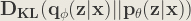
Now, let’s expand the KL Divergence:

$\mathbf{ D_{KL}(q_{\phi }(z|x)||p_{\theta }(z|x)) }$

$\mathbf{ = \int q_{\phi }(z|x)\log\frac{q_{\phi }(z|x)}{p_{\theta }(z|x)}dz }$

$\mathbf{ = \int q_{\phi }(z|x)\log\frac{q_{\phi }(z|x)p_{\theta }(x)}{p_{\theta }(z,x)}dz }$

$\mathbf{ = \int q_{\phi }(z|x)[\log p_{\theta }(x) + \log\frac{q_{\phi }(z|x)}{p_{\theta }(z,x)}]dz }$

$\mathbf{ = \int q_{\phi }(z|x)\log p_{\theta }(x)dz + \int q_{\phi }(z|x)\log\frac{q_{\phi }(z|x)}{p_{\theta }(z,x)}dz }$

$\mathbf{ = \log p_{\theta }(x) + \int q_{\phi }(z|x)\log\frac{q_{\phi }(z|x)}{p_{\theta }(x|z)p_{\theta }(z)}dz }$

$\mathbf{ = \log p_{\theta }(x) + \int q_{\phi }(z|x)[\log\frac{q_{\phi }(z|x)}{p_{\theta }(z)} - \log p_{\theta }(x|z)]dz }$

$\mathbf{ = \log p_{\theta }(x) + \int q_{\phi }(z|x)\log\frac{q_{\phi }(z|x)}{p_{\theta }(z)}dz - \int q_{\phi }(z|x)\log p_{\theta }(x|z)dz }$

$\mathbf{ = \log p_{\theta }(x) + E_{z\sim q_{\phi }(z|x)}\log\frac{q_{\phi }(z|x)}{p_{\theta }(z)} - E_{z\sim q_{\phi }(z|x)}\log p_{\theta }(x|z) }$

$\mathbf{ = \log p_{\theta }(x) + D_{KL}(q_{\phi }(z|x)||p_{\theta }(z)) - E_{z\sim q_{\phi }(z|x)}\log p_{\theta }(x|z) }$

$\mathbf{ \Rightarrow \log p_{\theta }(x) - D_{KL}(q_{\phi }(z|x)||p_{\theta }(z|x))) = E_{z\sim q_{\phi }(z|x)}\log p_{\theta }(x|z) - D_{KL}(q_{\phi }(z|x)||p_{\theta }(z)) }$

The L.H.S. consists of the terms we want to maximize:

The log-likelihood of generating real data: $\mathbf{ \log p_{\theta}(x) }$
Negative of the difference between the real and estimated posterior distribution: the $\mathbf{ D_{KL} }$ term.

The R.H.S. is called the evidence lower bound (ELBO) as it is always <= $\mathbf{\log p_{\theta}(x)}$ . This is because the KL Divergence is always non-negative.

The loss function will be the negative of the ELBO (as we minimize the loss and ELBO is maximized).

$\mathbf{ Loss(\theta, \phi ) = -E_{z\sim q_{\phi }(z|x)}\log p_{\theta }(x|z) + D_{KL}(q_{\phi }(z|x)||p_{\theta }(z)) }$

To see how to find the solution of the $\mathbf{D_{KL}}$ term and implement it in code for the case of a normal distribution, look at the appendix of this post.

Technical Details for Implementing VAE

This section will be for highlighting some of the technical details of using VAEs in practice. We’ll assume that the prior, $\mathbf{ p_{\theta }(z) }$ , follows a multivariate normal distribution.

The recognition model is a neural network that will output two vectors; one for the mean and the other for the standard deviation of the multivariate normal distribution of the latent space. One assumption imposed is that the covariance matrix of the multivariate normal distribution only has non-zero values on the diagonal, i.e. it is a diagonal matrix and hence a single vector is sufficient to describe it.

The generation model, also a neural network, will generate a reconstruction by sampling from the defined distribution. However, this sampling process introduces a major problem. Stochastic gradient descent via backpropagation cannot handle such stochastic units within the network! The sampling step blocks gradients from flowing into the recognition model and hence it will not train. To solve this problem, the “reparameterization trick” is used.

The Reparameterization Trick

The random variable $\mathbf{ z }$ is expressed as a deterministic variable $\mathbf{ z = g_{\phi }(\epsilon, x) }$ , where $\mathbf{ \epsilon }$ is an auxiliary independent random variable and $\mathbf{ g_{\phi } }$ , parametrized by $\mathbf{ \phi }$ , converts $\mathbf{ \epsilon }$ to $\mathbf{ z }$ .

The stochasticity only remains in the random variable $\mathbf{ \epsilon }$ , allowing the gradients to propagate into the recognition model (as $\mathbf{ \mu }$ and $\mathbf{ \sigma }$ are deterministic vectors).

As we have considered the distribution to be a multivariate normal with diagonal covariance structure, the reparameterization trick will give:

$\mathbf{z = \mu + \sigma \odot \epsilon}$ , where $\mathbf{\epsilon\sim N(0, I))}$

$\mathbf{z\sim q_{\phi }(z|x^{(i)}) = N(\mathbf{z}; \mu ^{(i)}, \sigma ^{2(i)}I)}$

Another small point to take care of is the fact that the network may learn negative values for $\mathbf{\sigma }$ . To prevent this, we can make the network learn $\mathbf{ \log \sigma }$ instead, and exponentiate this value to get the latent distribution’s standard deviation.

Generating New Data from Variational Autoencoders

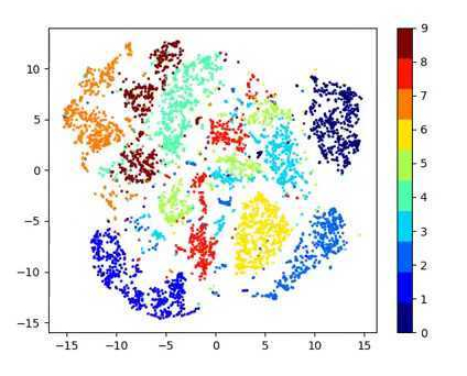
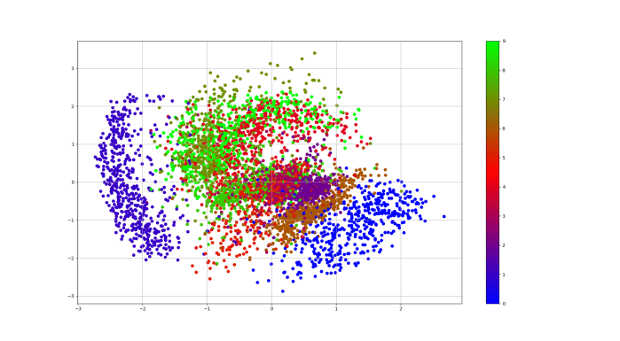
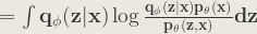
By sampling from the latent space and passing this to the generation model, we can generate new unseen data. As we had assumed the prior distribution, $\mathbf{ p_{\theta }(z) }$ , to be a unit normal distribution: $\mathbf{ z\sim N(0, \mathbf{I}) }$ .

I trained a variational autoencoder on the MNIST dataset for 20 epochs. The code can be found in this GitHub repo. The figure below shows the visualization of the 2D latent manifold. To generate this, a grid of encodings is sampled from the prior and passed as input to the generation model.

vae_Epoch20 — *2D latent manifold for MNIST.*

The visualization clearly shows how the encoding of the digits vary in the latent space and how different digits merge together (interpolation).

Mohit Jain

References

[1] Kingma, D. P. & Welling, M. (2013). Auto-Encoding Variational Bayes. CoRR, abs/1312.6114.

[2] Carl Doersch. Tutorial on variational autoencoders. arXiv:1606.05908, 2016.

[3] Intuitively Understanding Variational Autoencoders. Towards Data Science medium.

[4] From Autoencoders to Beta-VAE. lilianweng.github.io

[5] Variational autoencoders. jeremyjordan.me

[6] Ali Ghodsi: Deep Learning, Variational Autoencoder (Oct 12 2017)

[7] Variational Autoencoders. Arxiv Insights.

[8] Kullback-Leibler Divergence Explained. Count Bayesie

Appendix

Solution of $\mathbf{D_{KL}(q_{\phi}(z)||p_{\theta}(z))}$

We’ll assume that $q_{\phi}(z)$ and $p_{\theta}(z)$ are one dimensional Gaussian, i.e.

$q_{\phi}(z)\sim N(\mu, \sigma ^{2})$ and $p_{\theta}(z)\sim N(0, 1)$

Also, make note of the following properties as these will be used in derivation:

$p(x)\sim N(\mu, \sigma ^{2})$

$\int p(x)dx = 1$

$\int xp(x)dx = \mu$

$\int (x - \mu)^{2}p(x)dx = \sigma ^{2}$

Now, let’s move onto the derivation.

$D_{KL}(q_{\phi}(z)||p_{\theta}(z))$

$= \int q_{\phi}(z)\log\frac{q_{\phi}(z)}{p_{\theta}(z)}dz$

$= \int q_{\phi}(z)\log q_{\phi}(z)dz - \int q_{\phi}(z)\log p_{\theta}(z)dz\; \; \; ... \;(1)$

Now, taking the first term of (1):

$\int q_{\phi}(z)\log q_{\phi}(z)dz$

$= \int q_{\phi}(z)\log\frac{1}{(2\pi \sigma ^{2})^{\frac{1}{2}}}e^{-\frac{(z - \mu)^{2}}{2\sigma^{2}}}dz$

$= \int q_{\phi}(z)[-\frac{(z - \mu)^{2}}{2\sigma^{2}} - \log(2\pi \sigma ^{2})^\frac{1}{2}]dz$

$= -(\frac{1}{2\sigma ^{2}}\int (z - \mu)^{2}q_{\phi}(z)dz + \frac{1}{2}\log(2\pi \sigma ^{2})\int q_{\phi}(z)dz)$

$= -(\frac{1}{2\sigma ^{2}}.\sigma ^{2} + \frac{1}{2}\log(2\pi \sigma ^{2}).1)$

$= -\frac{1}{2}(1 + \log(2\pi \sigma ^{2}))\; \; \; ... \; (i)$

Now, taking the second term of (1):

$- \int q_{\phi}(z)\log p_{\theta}(z)dz$

$= -\int q_{\phi}(z)\log \frac{1}{(2\pi)^\frac{1}{2}}e^{-\frac{z^{2}}{2}}dz$

$= -\int q_{\phi}(z)[-\frac{z^{2}}{2} - \frac{1}{2}\log(2\pi)]dz$

$= \frac{1}{2}(\int z^{2}q_{\phi}(z)dz + \log(2\pi)\int q_{\phi}(z)dz)$

$= \frac{1}{2}(\int [(z - \mu)^{2} + 2\mu z - \mu ^{2}]q_{\phi}(z)dz + \log(2\pi).1)$

$= \frac{1}{2}(\int (z - \mu)^{2}q_{\phi}(z)dz + 2\mu \int zq_{\phi}(z)dz - \mu ^{2}\int q_{\phi}(z)dz + \log(2\pi))$

$= \frac{1}{2}(\sigma ^{2} + 2\mu ^{2} - \mu ^{2} + \log 2\pi)$

$= \frac{1}{2}(\sigma ^{2} + \mu ^{2} + \log 2\pi)\; \; \; ...\; (ii)$

Now, adding (i) and (ii),

$= -\frac{1}{2}(1 + \log(2\pi \sigma ^{2})) + \frac{1}{2}(\sigma ^{2} + \mu ^{2} + \log 2\pi)$

$\Rightarrow D_{KL}(q_{\phi}(z)||p_{\theta}(z)) = -\frac{1}{2}(\mu ^{2} + \sigma ^{2} - \log \sigma ^{2} - 1)$

The above derivation for the one dimensional case can easily by extended to the multivariate normal distribution. The expression then becomes:

$\mathbf{D_{KL}(q_{\phi}(z)||p_{\theta}(z)) = -\frac{1}{2}\sum_{k=1}^{K}((\mu _{k}) ^{2} + (\sigma _{k}) ^{2} - \log (\sigma _{k}) ^{2} - 1)}$

where $\mathbf{K}$ is the dimensionality of $\mathbf{z}$ and,

$\mathbf{q_{\phi}(z)\sim N(\mu, \sigma ^{2})}$ and $\mathbf{p_{\theta}(z)\sim N(0, I)}$

When using a recognition model $\mathbf{q_{\phi}(z|x)}$ then $\mathbf{\mu}$ and $\mathbf{\sigma}$ are simply functions of $\mathbf{x}$ and the variational parameters $\mathbf{\phi}$ . The above derived expression is used to implement the latent loss in code.

Code for the latent loss in TensorFlow:


#KL Divergence loss term

#The recognition model outputs log of the s.d.

#Exponentiate this to get actual s.d.

self.latent_loss = 0.5 * tf.reduce_sum(tf.square(self.z_mean) + tf.exp(2.0*z_stddev) - 2.0*z_stddev - 1, 1)

4 thoughts on “Variational Autoencoder Explained”

Pingback: The Intuition Behind Variational Autoencoders – Abacus.AI
Pingback: The Intuition Behind Variational Autoencoders – RealityEngines.AI
ale says:

February 2, 2019 at 4:43 pm

I’ve seen about 10 different explanations of the VAE but yours was the first where I understood why they made it generate a mean and a variance. Thank you!

LikeLiked by 1 person

1. natsu6767 says:
  
  February 2, 2019 at 10:07 pm
  
  Hi ale,
  Thanks for reading. Happy that the article helped you!
  
  LikeLike

Variational Autoencoder Explained

A Glance at Autoencoders

Variational Autoencoders to the Rescue

So, how does this help?

Mathematics Behind VAE

Technical Details for Implementing VAE

The Reparameterization Trick

Generating New Data from Variational Autoencoders

Mohit Jain

Appendix

Published by Natsu

4 thoughts on “Variational Autoencoder Explained”

Leave a comment Cancel reply

A Glance at Autoencoders

Variational Autoencoders to the Rescue

So, how does this help?

Mathematics Behind VAE

Technical Details for Implementing VAE

The Reparameterization Trick

Generating New Data from Variational Autoencoders

Mohit Jain

Appendix

Share this:

Related

Published by Natsu

4 thoughts on “Variational Autoencoder Explained”

Leave a comment Cancel reply