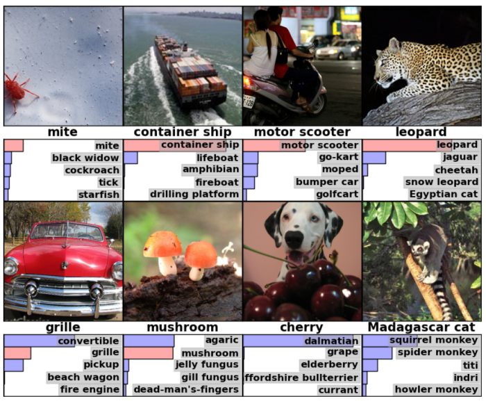
AlexNet famously won the 2012 ImageNet LSVRC-2012 competition by a large margin (15.3% VS 26.2% (second place) top-5 test error rates). This started the era of deep learning, bringing neural networks back into the spotlight!
Problems the paper addressed
To show that it is possible to successfully train a deep CNN with a large number of parameters (60 million) on the large ImageNet dataset in a reasonable amount of time and also achieve really good accuracy (even good enough to win the ImageNet LSVRC-2012 competition!).
To see how AlexNet was able to achieve this, let’s dive into its architecture!
AlexNet Architecture
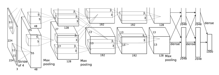
The net contains eight layers with weights; the first five are convolutional and the remaining three are fully-connected. The output of the last fully-connected layer is fed to a 1000-way softmax which produces a distribution over the 1000 class labels. The response-normalization layers follow the first and second convolutional layers. Max-pooling layers follow both of the response-normalization layers as well as the last (fifth) convolutional layer. The ReLU non-linearity is applied to the output of every convolutional and fully-connected layer.
The input to the net is a 227 × 227 × 3 image. The filters for each convolutional layers are:
- 96 kernels of size 11 × 11 × 3 with step size 4
- 256 kernels of size 5 × 5 × 48* with step size 1
- 384 kernels of size 3 × 3 × 256 with step size 1
- 384 kernels of size 3 × 3 × 192* with step size 1
- 256 kernels of size 3 × 3 × 192* with step size 1
* The discrepancy in the 3rd dimension of the filter sizes is because of the complex training procedure used to train AlexNet due to lack computational power. The net was spread across two GPUs and trained in parallel using complex connections. This is no longer required to train AlexNet due to the availability of better GPUs.
Now let’s look at the new layers that were introduced in AlexNet:
ReLU Nonlinearity
The standard non-linearity used so far are Tanh or Sigmoid non-linearity. But the problem with them is that they have “saturating regions”. These are regions where the gradient becomes very small. As a result gradient descent becomes very slow and training takes longer. There is only a very small pocket where these functions give large enough gradient to make training progress faster.
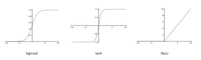
ReLU, ƒ(x) = max(0, x), takes care of this gradient problem (for the positive portion). Though, the gradient does become zero for negative values, it has been found that this doesn’t cause much of a problem and experimentally it has been found that using ReLU speeds up the training by a significant amount. You get a rough speed up of a factor of 6 using ReLU for the same accuracy.
Local Response Normalization
This layer boosted the accuracy of the net and also helps in generalization.
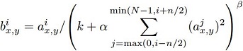
a(i, x, y) represents the ith conv. kernel’s output (after ReLU) at the position of (x, y) in the feature map.
b(i, x, y) represents the ith output of local response normalization, and is also the input for the next layer.
N is the total number of the conv. kernels in the layer.
n is the number of “adjacent” conv. kernel maps (in the paper n = 5).
k, α, β are hyper-parameters (in the paper k = 2, α = 10e-4, β = 0.75).
In the paper it is mentioned that response normalization is a form of lateral inhibition inspired by the type found in real neurons. Local response normalization (LRN) is no longer used in artificial neural networks as better alternatives are present. There isn’t much intuition or reasoning for the use of LRN given in the paper other than that, that it helped reduced the error. An intuition I came up with (not perfect) is:
Say, there are six kernels which will be responsible (as initially, before training, all the kernels are random and not good at detecting a particular feature) for detecting the four corner (top-left, top-right, bottom-left and bottom-right), edges and the middle of a table respectively. Say position (x, y) where the kernels are applied is a top-left corner of a table in the image. The activity of the neuron computed by the kernel responsible for the top left corner should be high. LRN enforces this by creating a competition, making the neurons with big activities give bigger activities as compared to those with lower activation. As a result, after training the kernel with the highest activation for a top-left corner will become better at detecting it as compared to other kernels.
The above intuition isn’t the best. If you find a flaw or have a better intuition please mention it.
Check out this article for more info: Normalizations in Neural Networks
Overlapping Pooling
Traditionally pooling regions did not overlap. This paper changed the conventional idea of pooling by making the pooling regions overlap. Say, the pooling region is z × z, the step size of the filter, s < z. Doing this reduced the error and made it more difficult for the model to overfit.
Training
The model was trained using stochastic gradient descent with a batch size of 128 examples, momentum of 0.9 and weight decay of 0.0005. The learning rate was initialized at 0.01 and reduced by 10 when the validation error rate plateaued.
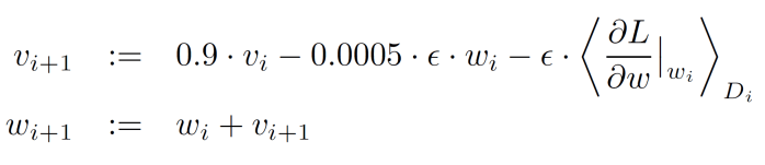
i is the iteration index
υ is the momentum variable
∈ is the learning rate
(∂L / ∂w | w(i)) is the average over the ith batch D(i) of the derivative of the objective with respect to w, evaluated at w(i).
To prevent the model from overfitting, two methods are used:
Data Augmentation
Two types of data augmentation are used. First involves extracting random 227 × 227 patches (and their horizontal reflections) from the 256 × 256 images an training the network on these extracted patches. This increases the effective number of training examples. The second involves performing PCA on the set of RGB pixel values throughout the ImageNet training set. Doing this approximately captures an important property of natural images: object identity is invariant to changes in the intensity and color of the illumination.
Dropout
This was the first paper to use droput to reduce overfitting. Dropout consists
of setting to zero the output of each hidden neuron with probability p (p = 0.5 in the paper). The neurons which are “dropped out” in this way do not contribute to the forward pass and do not participate in backpropagation. So every time an input is presented, the neural network randomly samples a different architecture, but all these architectures share weights! As a result of this, it forces each neuron to rely less, and thus form complex dependencies, on other neurons forcing it to learn more robust features that are useful in conjunction with many different random subsets of the other neurons.
At test time all the neurons are used but their outputs are multiplied by the dropout probability p. In AlexNet, dropout is used in the first two fully-connected layers (layers 6 & 7).
Conclusion
This paper was a breakthrough in the field of computer vision. It helped show that artificial neural networks weren’t doomed as they were thought to be and sparked the beginning of the cutting-edge research happening in deep learning all over the world!
Original paper: Imagenet Classification with Deep Convolutional Neural Networks
Implementation of AlexNet (Modified): https://github.com/Natsu6767/Modified-AlexNet-Tensorflow
